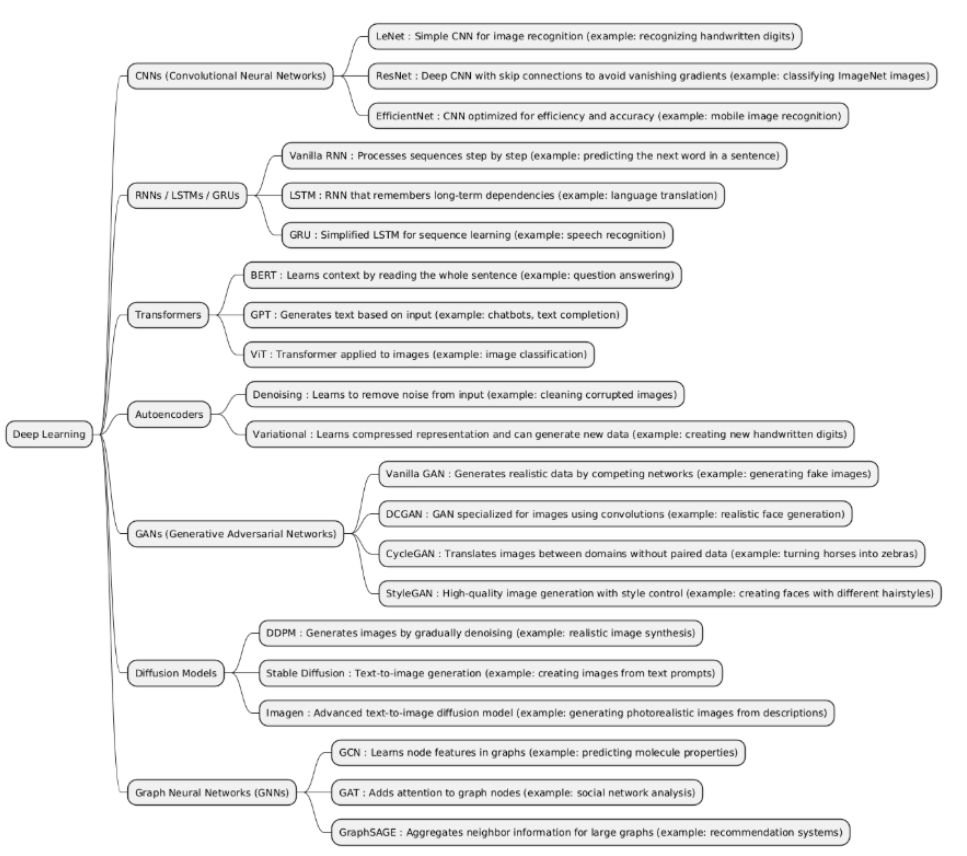
Deep Learning is a subfield of machine learning that uses neural networks with many layers to model complex patterns in data. It is especially powerful for tasks like image recognition, natural language processing, and speech recognition, where traditional algorithms struggle to achieve high accuracy.
| Type | What it is | When it is used | When it is preferred over other types | When it is not recommended | Examples of projects that is better use it incide him |
|---|---|---|---|---|---|
| CNNs | Convolutional Neural Networks (CNNs) are deep learning models designed to process grid-like data, especially images. They use convolutional layers to automatically extract spatial features. | Used for tasks where spatial hierarchies are important, such as image recognition, object detection, segmentation, and video frame analysis. |
• Better than RNNs, LSTMs, GRUs for static spatial data (images) instead of sequences. • Better than Transformers for smaller image datasets where computational cost matters. • Better than Autoencoders/GANs/Diffusion Models when the goal is discriminative tasks (classification/detection) rather than generation. • Better than Graph Neural Networks when data is regular grids rather than graph-structured. |
• Not suitable for sequential or time-series data — RNNs/LSTMs/Transformers are better. • Not ideal for graph-structured data — use GNNs. • Not optimal for complex generative tasks — GANs or Diffusion Models are better. |
• Image classification (e.g., MNIST, CIFAR-10). • Object detection (e.g., YOLO, Faster R-CNN). • Medical image segmentation (e.g., detecting tumors in MRI scans). |
| RNNs, LSTMs, GRUs | RNNs, LSTMs, and GRUs are sequence-processing deep learning models. • RNNs: basic recurrent networks that maintain hidden states to process sequences. • LSTMs: RNNs with input, forget, and output gates to capture long-term dependencies. • GRUs: simplified LSTMs with fewer gates (reset and update), faster to train but also capture long-term dependencies. |
Used for sequential or time-series data such as text, speech, audio, or sensor readings. |
• Better than CNNs for data with temporal or sequential dependencies. • Better than Autoencoders for sequence prediction tasks. • Can be better than Transformers for short-to-medium sequences with limited computational resources. • Not used for pure generative image tasks (use GANs or Diffusion Models) or graph-structured data (use GNNs). |
• For very long sequences, Transformers are more effective. • For non-sequential or grid-structured data, CNNs or GNNs are better. • For large-scale parallel training, Transformers are faster. |
• Text generation (predicting next words in sentences). • Speech recognition (audio-to-text conversion). • Time-series forecasting (stock prices, weather, sensor data). • Anomaly detection in sequences (equipment monitoring or network traffic). |
| Transformers | Transformers are deep learning models that rely on self-attention mechanisms to process data, capturing long-range dependencies without recurrence. They are highly parallelizable and excel at sequence modeling. | Used for tasks involving sequential data, language, vision, or multimodal inputs. Common in NLP, text generation, translation, and image processing (Vision Transformers). |
• Better than RNNs/LSTMs/GRUs when handling long sequences, as they avoid vanishing gradient issues. • Better than CNNs for tasks requiring global context rather than local features only. • Better than Autoencoders/GANs/Diffusion Models for discriminative or generative sequence tasks. • Better than Graph Neural Networks for unstructured sequential or token-based data rather than graph-structured data. |
• When dataset is very small — Transformers require large amounts of data to perform well. • When computational resources are limited — Transformers are resource-intensive. • For purely grid-based tasks with small local context — CNNs may be simpler and faster. |
• Language modeling and text generation (e.g., GPT, BERT). • Machine translation (e.g., English to French). • Vision Transformers for image classification. • Multimodal tasks like text-to-image generation (e.g., DALL·E). |
| Autoencoders | Autoencoders are deep learning models that learn to compress data into a latent representation (encoding) and then reconstruct it back (decoding). They are unsupervised/self-supervised and focus on learning efficient data representations. | Used for dimensionality reduction, denoising, anomaly detection, and representation learning. |
• Better than CNNs/RNNs/LSTMs/GRUs/Transformers when the goal is unsupervised feature learning or compression, not sequence modeling or discriminative tasks. • Better than GANs/Diffusion Models for simpler reconstruction tasks rather than generative data creation. • Better than Graph Neural Networks when data is non-graph structured. |
• Not ideal for complex generative tasks — GANs or Diffusion Models are better. • Not optimal for sequence prediction or classification — use RNNs, Transformers, or CNNs. • Representations may not be discriminative enough for downstream tasks. |
• Image denoising autoencoder — removing noise from images. • Anomaly detection — detecting unusual patterns in manufacturing sensor data. |
| GANs | Generative Adversarial Networks (GANs) are deep learning models consisting of two networks — a generator and a discriminator — that compete. The generator creates synthetic data, and the discriminator evaluates its authenticity, enabling realistic data generation. | Used for data generation, image synthesis, style transfer, super-resolution, and augmentation. |
• Better than Autoencoders when you want high-quality realistic generation rather than simple reconstruction. • Better than CNNs/RNNs/LSTMs/Transformers when the task is generative rather than discriminative. • Better than Diffusion Models for faster generation (though diffusion models may produce higher fidelity). • Not directly comparable with Graph Neural Networks unless generating graph data. |
• When you only need representation learning or compression — Autoencoders suffice. • When dataset is very small — GANs can be unstable. • When stable training is critical — GANs are prone to mode collapse. • For tasks requiring sequence modeling — use RNNs, LSTMs, or Transformers instead. |
• Image generation — generating human faces (e.g., StyleGAN). • Image-to-image translation — converting sketches to photos. • Super-resolution — enhancing image resolution. |
| Diffusion Models | Diffusion Models are deep generative models that learn to generate data by reversing a gradual noise process. They start from random noise and iteratively denoise it to produce realistic samples. | Used for high-fidelity image generation, text-to-image synthesis, and complex data generation tasks. |
• Better than GANs for generating more diverse and high-quality samples with fewer mode collapse issues. • Better than Autoencoders for realistic generative tasks rather than reconstruction. • Better than CNNs/RNNs/LSTMs/Transformers for generation rather than discriminative or sequential tasks. • Not directly comparable with Graph Neural Networks, unless generating graph-like data. |
• When fast generation is required — diffusion models are slower than GANs. • When dataset is small — training can be difficult. • When task is discriminative (classification, detection) — CNNs or Transformers are better. |
• Text-to-image generation (e.g., DALL·E 2, Stable Diffusion). • High-resolution image synthesis from noise. • Image inpainting — filling missing parts of images. • Video generation or frame interpolation. |
| GNNs | Graph Neural Networks (GNNs) are deep learning models designed to work with graph-structured data, where nodes represent entities and edges represent relationships. They learn node, edge, or graph-level embeddings by aggregating information from neighbors. | Used when data is non-Euclidean or naturally represented as a graph, such as social networks, molecular structures, knowledge graphs, or transportation networks. |
• Better than CNNs/RNNs/LSTMs/Transformers for relational or graph-structured data. • Better than Autoencoders/GANs/Diffusion Models for tasks that require node classification, link prediction, or graph-level prediction rather than pure generative tasks. |
• When data is grid-like (images) — CNNs are simpler. • When data is sequential — RNNs, LSTMs, or Transformers are better. • When generative modeling of images/audio is the goal — GANs or Diffusion Models are better. |
• Node classification in social networks (e.g., predicting user interests). • Molecule property prediction in chemistry or drug discovery. • Link prediction for recommendation systems (e.g., predicting friendships). |
import torch
import torch.nn as nn
import torchvision
import torchvision.transforms as transforms
from sklearn.semi_supervised import LabelPropagation
from sklearn.metrics import accuracy_score
import numpy as np

# 1️⃣ Load CIFAR-10 subset
transform = transforms.Compose([
    transforms.Resize((32, 32)),
    transforms.ToTensor()
])

dataset = torchvision.datasets.CIFAR10(root='./data', train=True, download=True, transform=transform)
loader = torch.utils.data.DataLoader(dataset, batch_size=64, shuffle=True)

# 2️⃣ Use pretrained ResNet18 as feature extractor
resnet = torchvision.models.resnet18(weights=torchvision.models.ResNet18_Weights.DEFAULT)
resnet.fc = nn.Identity()
resnet.eval()

# 3️⃣ Extract embeddings for first N images
N = 20
X_list = []
y_list = []
for i, (imgs, labels) in enumerate(loader):
    with torch.no_grad():
        embeddings = resnet(imgs).numpy()
        X_list.append(embeddings)
        y_list.append(labels.numpy())
    if len(X_list)*64 >= N:
        break

X = np.vstack(X_list)[:N]
y = np.hstack(y_list)[:N]

# 4️⃣ Make some labels unknown (-1)
y_semi = y.copy()
y_semi[10:] = -1

# 5️⃣ Apply Label Propagation
label_prop_model = LabelPropagation()
label_prop_model.fit(X, y_semi)
predicted_labels = label_prop_model.transduction_

# 6️⃣ Evaluate
accuracy = accuracy_score(y, predicted_labels)
print("Predicted labels:", predicted_labels)
print("Accuracy:", accuracy)
import torch
import torch.nn as nn
from sklearn.semi_supervised import LabelPropagation
from sklearn.metrics import accuracy_score
import numpy as np

# 1️⃣ Example sequence dataset
sequences = [
    "I love machine learning",
    "Python is great",
    "I hate bugs",
    "Debugging is frustrating",
    "AI is the future",
    "I dislike slow computers"
]

# Labels: 1 = positive, 0 = negative, -1 = unlabeled
labels = np.array([1, 1, 0, 0, -1, -1])

# 2️⃣ Tokenize sequences
word_to_idx = {}
for seq in sequences:
    for word in seq.lower().split():
        if word not in word_to_idx:
            word_to_idx[word] = len(word_to_idx)
vocab_size = len(word_to_idx)
max_len = max(len(seq.split()) for seq in sequences)

def encode(seq):
    tokens = [word_to_idx[w] for w in seq.lower().split()]
    tokens += [0]*(max_len - len(tokens))
    return tokens

X_seq = np.array([encode(seq) for seq in sequences])

# 3️⃣ Define simple LSTM encoder
class LSTMEncoder(nn.Module):
    def __init__(self, vocab_size, embed_dim=10, hidden_dim=4):
        super().__init__()
        self.embedding = nn.Embedding(vocab_size, embed_dim, padding_idx=0)
        self.lstm = nn.LSTM(embed_dim, hidden_dim, batch_first=True)
    def forward(self, x):
        x = self.embedding(x)
        _, (h_n, _) = self.lstm(x)
        return h_n.squeeze(0)

model = LSTMEncoder(vocab_size)
model.eval()

# 4️⃣ Get embeddings
with torch.no_grad():
    X_emb = model(torch.tensor(X_seq)).numpy()

# 5️⃣ Apply Label Propagation
label_prop = LabelPropagation()
label_prop.fit(X_emb, labels)
predicted_labels = label_prop.transduction_

# 6️⃣ Evaluate
true_labels = np.array([1, 1, 0, 0, 1, 0])
accuracy = accuracy_score(true_labels, predicted_labels)
print("Predicted labels:", predicted_labels)
print("Accuracy:", accuracy)
import numpy as np
from sklearn.semi_supervised import LabelPropagation
from sklearn.metrics import accuracy_score
from transformers import AutoTokenizer, AutoModel
import torch

# 1️⃣ Example text data
texts = [
    "I love machine learning",
    "Python is great for AI",
    "I hate bugs in code",
    "Debugging is frustrating",
    "AI is the future",
    "I dislike slow computers"
]

# Labels: 1 = positive, 0 = negative, -1 = unlabeled
labels = np.array([1, 1, 0, 0, -1, -1])

# 2️⃣ Load GPT-like model
tokenizer = AutoTokenizer.from_pretrained("distilgpt2")
model = AutoModel.from_pretrained("distilgpt2")
model.eval()

# 3️⃣ Encode text into embeddings
def get_embedding(text):
    inputs = tokenizer(text, return_tensors="pt")
    with torch.no_grad():
        outputs = model(**inputs)
    return outputs.last_hidden_state.mean(dim=1).squeeze().numpy()

X = np.array([get_embedding(t) for t in texts])

# 4️⃣ Apply Label Propagation
label_prop_model = LabelPropagation()
label_prop_model.fit(X, labels)
predicted_labels = label_prop_model.transduction_

# 5️⃣ Evaluate
true_labels = np.array([1, 1, 0, 0, 1, 0])
accuracy = accuracy_score(true_labels, predicted_labels)
print("Predicted labels:", predicted_labels)
print("Accuracy:", accuracy)
import torch
from diffusers import StableDiffusionPipeline
from sklearn.semi_supervised import LabelPropagation
from sklearn.metrics import accuracy_score
import numpy as np
from PIL import Image

# 1️⃣ Example text prompts
texts = [
    "A cute puppy",
    "A sunny beach",
    "A scary monster",
    "A dark forest",
    "A happy child",
    "A rainy city"
]

# Labels: 1 = positive, 0 = negative, -1 = unlabeled
labels = np.array([1, 1, 0, 0, -1, -1])

# 2️⃣ Load Stable Diffusion pipeline
pipe = StableDiffusionPipeline.from_pretrained("runwayml/stable-diffusion-v1-5", torch_dtype=torch.float32)
pipe.to("cpu")
text_encoder = pipe.text_encoder
tokenizer = pipe.tokenizer

# 3️⃣ Encode text prompts into embeddings
def get_embedding(text):
    inputs = tokenizer(text, return_tensors="pt")
    with torch.no_grad():
        outputs = text_encoder(**inputs)
    return outputs.last_hidden_state.mean(dim=1).squeeze().numpy()

X = np.array([get_embedding(t) for t in texts])

# 4️⃣ Apply Label Propagation
label_prop_model = LabelPropagation()
label_prop_model.fit(X, labels)
predicted_labels = label_prop_model.transduction_

# 5️⃣ Evaluate
true_labels = np.array([1, 1, 0, 0, 1, 0])
accuracy = accuracy_score(true_labels, predicted_labels)
print("Predicted labels:", predicted_labels)
print("Accuracy:", accuracy)